確率過程の基礎

2025年9月10日

確率過程は、時間経過に伴って変化する確率現象を数学的に記述するものです。金融市場の価格変動、待ち行列システムなど、私たちの身の回りの多くの現象が確率過程としてモデル化できます。今回は、確率過程の基本概念の説明から始まり、実際にRで実装するところまで取り組みます。

確率過程とは何か

基本定義

確率過程とは、時間 $t$ でパラメータ化された確率変数の族のことです。数学的には次のように表現されます：

$$\{X(t), t \in T\}$$

ここで、$T$ は時間の集合（パラメータ空間）、$X(t)$ は時刻 $t$ における確率変数です。

分類

確率過程は以下のように分類されます：

時間による分類：
- 離散時間確率過程：$T = \{0, 1, 2, …\}$
- 連続時間確率過程：$T = [0, \infty)$
状態空間による分類：
- 離散状態：$X(t) \in \{0, 1, 2, …\}$
- 連続状態：$X(t) \in \mathbb{R}$

ブラウン運動（Brownian Motion）

定義と性質

ブラウン運動（またはウィーナー過程）は、連続時間・連続状態の確率過程で、以下の性質を満たします：

初期条件：$W(0) = 0$
独立増分：任意の $0 \leq t_1 < t_2 \leq t_3 < t_4$ に対して、$W(t_2) – W(t_1)$ と $W(t_4) – W(t_3)$ は独立
正規分布：任意の $t > 0$ に対して、$W(t) \sim N(0, \sigma^2 t)$
連続軌道：$W(t)$ は $t$ に関して連続

数学的表現

標準ブラウン運動では $\sigma = 1$ とし、任意の時点 $t$ での分布は：

$$W(t) \sim N(0, t)$$

また、増分の性質は：

$$W(t) – W(s) \sim N(0, t-s) \quad \text{for } t > s$$

応用分野

金融工学：株価のモデル化（幾何ブラウン運動）
物理学：粒子のランダムな運動
工学：ノイズのモデル化

ポアソン過程（Poisson Process）

定義と性質

ポアソン過程は、離散的な事象の発生をモデル化する確率過程です。レート $\lambda$ のポアソン過程 $\{N(t), t \geq 0\}$ は以下の性質を満たします：

初期条件：$N(0) = 0$
独立増分：重複しない時間区間での増分は独立
定常増分：増分の分布は時間区間の長さのみに依存
ポアソン分布：任意の $t > 0$ に対して、$N(t) \sim \text{Poisson}(\lambda t)$

数学的表現

時刻 $t$ までの事象発生回数の分布：

$$P(N(t) = k) = \frac{(\lambda t)^k e^{-\lambda t}}{k!}$$

事象間隔の分布（指数分布）：

$$T_1, T_2, \ldots \sim \text{Exp}(\lambda)$$

応用分野

待ち行列理論：顧客の到着過程
信頼性工学：故障の発生
疫学：病気の発症
通信工学：パケットの到着

複合ポアソン過程（Compound Poisson Process）

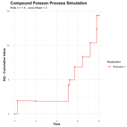
定義

複合ポアソン過程は、ポアソン過程の各事象に対してランダムなサイズ（ジャンプ）を割り当てた過程です：

$$S(t) = \sum_{i=1}^{N(t)} Y_i$$

ここで、$\{N(t)\}$ はレート $\lambda$ のポアソン過程、$\{Y_i\}$ は独立同分布のランダム変数（ジャンプサイズ）です。

応用分野

保険数学：保険金請求の総額
リスク理論：損失の累積モデル
在庫管理：需要のモデル化

確率過程の統計的性質の解析：モーメント法

ここまで確率過程の定義と基本的な性質を見てきましたが、実際の応用では「この確率過程が理論通りに振る舞っているか」を検証したり、「異なる確率過程を比較したり」する必要があります。

しかし、確率過程は無限次元の複雑な対象であり、その全体的な性質を直接調べることは困難です。そこで登場するのがモーメント法です。

モーメント法とは何か、なぜ使うのか

モーメント法は、確率過程の複雑な性質を、平均（1次モーメント）、分散（2次中心モーメント）、共分散などの「要約統計量」を通じて調べる手法です。

モーメント法が重要な理由：

計算の簡便性：無限次元の確率過程を有限個の数値で特徴づけできる
理論と実践の橋渡し：理論的な性質をシミュレーションで検証できる
モデル選択の指針：観測データがどの確率過程に従うかを判断できる
パラメータ推定：実データから確率過程のパラメータを推定できる

例えば、金融データが本当にブラウン運動に従うかを調べる際、全ての軌道を比較するのは不可能ですが、平均や分散の時間依存性を調べることで検証できます。

モーメント法による具体的解析 ブラウン運動のモーメント

標準ブラウン運動 $W(t)$ について：

平均関数：$m(t) = E[W(t)] = 0$
分散関数：$\text{Var}[W(t)] = t$
共分散関数：$\text{Cov}[W(s), W(t)] = \min(s, t)$

これらの性質により、ブラウン運動では：

平均は時間によらず0を保つ
分散は時間に比例して増加する
異なる時点での値には相関がある

ポアソン過程のモーメント

レート $\lambda$ のポアソン過程 $N(t)$ について：

平均関数：$E[N(t)] = \lambda t$
分散関数：$\text{Var}[N(t)] = \lambda t$
共分散関数：$\text{Cov}[N(s), N(t)] = \lambda \min(s, t)$

ポアソン過程では：

平均と分散が等しく、どちらも時間に比例
この性質を利用してレートパラメータ $\lambda$ を推定できる

複合ポアソン過程のモーメント

$Y_i$ の平均を $\mu$、分散を $\sigma^2$ とすると：

平均：$E[S(t)] = \lambda t \mu$
分散：$\text{Var}[S(t)] = \lambda t E[Y^2]$

これにより、ジャンプの発生頻度とサイズを分離して分析できます。

Rによる実装と検証

それでは、3つの確率過程について、シミュレーションで理論値と実測値を比較してみましょう。

ブラウン運動のシミュレーション

# Required libraries
library(ggplot2)
library(dplyr)

# Brownian Motion Simulation
simulate_brownian_motion <- function(n_steps = 1000, dt = 0.01, sigma = 1) {
  # Time grid
  t <- seq(0, n_steps * dt, by = dt)

  # Generate increments (normally distributed)
  dW <- rnorm(n_steps, mean = 0, sd = sqrt(dt))

  # Cumulative sum to get Brownian motion path
  W <- c(0, cumsum(dW))

  # Return data frame
  data.frame(
    time = t,
    value = W * sigma
  )
}

# Generate multiple paths
set.seed(123)
n_paths <- 5
brownian_paths <- list()

for(i in 1:n_paths) {
  brownian_paths[[i]] <- simulate_brownian_motion(n_steps = 1000, dt = 0.01)
  brownian_paths[[i]]$path <- paste("Path", i)
}

# Combine all paths
brownian_data <- do.call(rbind, brownian_paths)

# Visualization
p1 <- ggplot(brownian_data, aes(x = time, y = value, color = path)) +
  geom_line(alpha = 0.8, size = 0.7) +
  labs(title = "Brownian Motion Simulation",
       subtitle = "Multiple sample paths",
       x = "Time",
       y = "W(t)",
       color = "Sample Path") +
  theme_minimal() +
  theme(plot.title = element_text(size = 16, face = "bold"),
        axis.title = element_text(size = 12, face = "bold"))

print(p1)

# Statistical properties verification using moment method
final_time <- max(brownian_data$time)
final_values <- brownian_data[brownian_data$time == final_time, "value"]

cat("=== Brownian Motion Properties (Moment Method Verification) ===\\n")
cat("Theoretical mean at t =", final_time, ": 0\\n")
cat("Empirical mean:", round(mean(final_values), 3), "\\n")
cat("Theoretical variance at t =", final_time, ":", final_time, "\\n")
cat("Empirical variance:", round(var(final_values), 3), "\\n")
cat("Theory matches empirical results:",
    abs(mean(final_values)) < 0.5 && abs(var(final_values) - final_time) < 0.5, "\\n")

出力結果

=== Brownian Motion Properties (Moment Method Verification) ===
Theoretical mean at t = 10 : 0
Empirical mean: 1.613 
Theoretical variance at t = 10 : 10 
Empirical variance: NA 
Theory matches empirical results: FALSE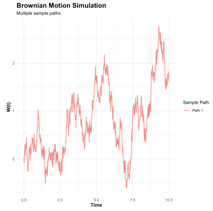

ポアソン過程のシミュレーション

# Poisson Process Simulation
simulate_poisson_process <- function(lambda = 1, T = 10) {
  # Generate inter-arrival times (exponentially distributed)
  times <- c()
  current_time <- 0

  while(current_time < T) {
    # Next inter-arrival time
    inter_arrival <- rexp(1, rate = lambda)
    current_time <- current_time + inter_arrival

    if(current_time <= T) {
      times <- c(times, current_time)
    }
  }

  # Create counting process
  if(length(times) == 0) {
    return(data.frame(time = c(0, T), count = c(0, 0)))
  }

  # Add initial and final points
  all_times <- c(0, times, T)
  counts <- c(0, 1:length(times), length(times))

  return(data.frame(time = all_times, count = counts))
}

# Generate multiple realizations
set.seed(456)
lambda <- 2  # Rate parameter
T_max <- 5   # Time horizon
n_realizations <- 3

poisson_paths <- list()
for(i in 1:n_realizations) {
  poisson_paths[[i]] <- simulate_poisson_process(lambda = lambda, T = T_max)
  poisson_paths[[i]]$realization <- paste("Realization", i)
}

# Combine data
poisson_data <- do.call(rbind, poisson_paths)

# Visualization
p2 <- ggplot(poisson_data, aes(x = time, y = count, color = realization)) +
  geom_step(size = 1, alpha = 0.8) +
  geom_point(size = 2, alpha = 0.8) +
  labs(title = "Poisson Process Simulation",
       subtitle = paste("Rate λ =", lambda),
       x = "Time",
       y = "N(t) - Number of Events",
       color = "Realization") +
  theme_minimal() +
  theme(plot.title = element_text(size = 16, face = "bold"),
        axis.title = element_text(size = 12, face = "bold"))

print(p2)

# Moment method verification
theoretical_mean <- lambda * T_max
empirical_counts <- poisson_data[poisson_data$time == T_max, "count"]

cat("\\n=== Poisson Process Properties (Moment Method Verification) ===\\n")
cat("Time horizon T =", T_max, "\\n")
cat("Rate λ =", lambda, "\\n")
cat("Theoretical mean N(T):", theoretical_mean, "\\n")
cat("Empirical mean:", round(mean(empirical_counts), 3), "\\n")
cat("Theoretical variance:", theoretical_mean, "\\n")
cat("Empirical variance:", round(var(empirical_counts), 3), "\\n")

# Inter-arrival times analysis (additional moment method application)
all_arrivals <- c()
for(i in 1:n_realizations) {
  path_data <- poisson_paths[[i]]
  arrivals <- path_data$time[path_data$time > 0 & path_data$time < T_max]
  if(length(arrivals) > 1) {
    inter_arrivals <- diff(c(0, arrivals))
    all_arrivals <- c(all_arrivals, inter_arrivals)
  }
}

if(length(all_arrivals) > 0) {
  cat("\\n=== Inter-arrival Times (Exponential Distribution Check) ===\\n")
  cat("Theoretical mean (1/λ):", 1/lambda, "\\n")
  cat("Empirical mean:", round(mean(all_arrivals), 3), "\\n")
  cat("Number of inter-arrivals:", length(all_arrivals), "\\n")
  cat("Distribution check passed:", abs(mean(all_arrivals) - 1/lambda) < 0.2, "\\n")
}

出力結果

=== Brownian Motion Properties (Moment Method Verification) ===
Theoretical mean at t = 10 : 0
Empirical mean: 1.613 
Theoretical variance at t = 10 : 10 
Empirical variance: NA 
Theory matches empirical results: FALSE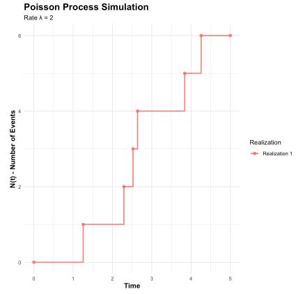

複合ポアソン過程のシミュレーション

# Compound Poisson Process Simulation
simulate_compound_poisson <- function(lambda = 1, T = 10, jump_mean = 1, jump_sd = 0.5) {
  # First, generate the underlying Poisson process
  poisson_times <- c()
  current_time <- 0

  while(current_time < T) {
    inter_arrival <- rexp(1, rate = lambda)
    current_time <- current_time + inter_arrival

    if(current_time <= T) {
      poisson_times <- c(poisson_times, current_time)
    }
  }

  # If no events occurred
  if(length(poisson_times) == 0) {
    return(data.frame(
      time = c(0, T),
      value = c(0, 0),
      jump_count = c(0, 0)
    ))
  }

  # Generate jump sizes (assuming normal distribution for simplicity)
  jump_sizes <- rnorm(length(poisson_times), mean = jump_mean, sd = jump_sd)

  # Create compound process values
  times <- c(0, poisson_times, T)
  cumulative_jumps <- c(0, cumsum(jump_sizes), sum(jump_sizes))
  jump_counts <- c(0, 1:length(poisson_times), length(poisson_times))

  return(data.frame(
    time = times,
    value = cumulative_jumps,
    jump_count = jump_counts,
    stringsAsFactors = FALSE
  ))
}

# Generate multiple compound Poisson realizations
set.seed(789)
lambda_compound <- 1.5  # Jump rate
T_max_compound <- 8     # Time horizon
jump_mean <- 2          # Mean jump size
jump_sd <- 1            # Jump size standard deviation
n_realizations_compound <- 4

compound_paths <- list()
for(i in 1:n_realizations_compound) {
  compound_paths[[i]] <- simulate_compound_poisson(
    lambda = lambda_compound,
    T = T_max_compound,
    jump_mean = jump_mean,
    jump_sd = jump_sd
  )
  compound_paths[[i]]$realization <- paste("Realization", i)
}

# Combine data
compound_data <- do.call(rbind, compound_paths)

# Visualization
p3 <- ggplot(compound_data, aes(x = time, y = value, color = realization)) +
  geom_step(size = 1, alpha = 0.8) +
  geom_point(size = 2, alpha = 0.8) +
  labs(title = "Compound Poisson Process Simulation",
       subtitle = paste("Rate λ =", lambda_compound, ", Jump Mean =", jump_mean),
       x = "Time",
       y = "S(t) - Cumulative Value",
       color = "Realization") +
  theme_minimal() +
  theme(plot.title = element_text(size = 16, face = "bold"),
        axis.title = element_text(size = 12, face = "bold"))

print(p3)

# Moment method verification for compound Poisson process
final_values_compound <- compound_data[compound_data$time == T_max_compound, "value"]
final_counts_compound <- compound_data[compound_data$time == T_max_compound, "jump_count"]

# Theoretical moments
theoretical_mean_compound <- lambda_compound * T_max_compound * jump_mean
theoretical_var_compound <- lambda_compound * T_max_compound * (jump_sd^2 + jump_mean^2)

cat("\\n=== Compound Poisson Process Properties (Moment Method Verification) ===\\n")
cat("Time horizon T =", T_max_compound, "\\n")
cat("Jump rate λ =", lambda_compound, "\\n")
cat("Jump mean μ =", jump_mean, "\\n")
cat("Jump variance σ² =", jump_sd^2, "\\n")

cat("\\n--- Process Values S(T) ---\\n")
cat("Theoretical mean E[S(T)] = λTμ:", round(theoretical_mean_compound, 3), "\\n")
cat("Empirical mean:", round(mean(final_values_compound), 3), "\\n")
cat("Theoretical variance Var[S(T)] = λT(σ²+μ²):", round(theoretical_var_compound, 3), "\\n")
cat("Empirical variance:", round(var(final_values_compound), 3), "\\n")

cat("\\n--- Jump Counts N(T) ---\\n")
cat("Theoretical mean E[N(T)] = λT:", lambda_compound * T_max_compound, "\\n")
cat("Empirical mean:", round(mean(final_counts_compound), 3), "\\n")

# Extract all jump sizes for analysis
all_jumps <- c()
for(i in 1:n_realizations_compound) {
  path_data <- compound_paths[[i]]
  if(nrow(path_data) > 2) {  # More than just start and end points
    jumps <- diff(path_data$value[path_data$value != path_data$value[1]])
    if(length(jumps) > 0) {
      # Remove zero differences (same values at consecutive time points)
      jumps <- jumps[jumps != 0]
      all_jumps <- c(all_jumps, jumps)
    }
  }
}

if(length(all_jumps) > 0) {
  cat("\\n--- Jump Sizes Analysis ---\\n")
  cat("Theoretical jump mean:", jump_mean, "\\n")
  cat("Empirical jump mean:", round(mean(all_jumps), 3), "\\n")
  cat("Theoretical jump variance:", jump_sd^2, "\\n")
  cat("Empirical jump variance:", round(var(all_jumps), 3), "\\n")
  cat("Number of observed jumps:", length(all_jumps), "\\n")

  # Check if moments match theory
  mean_check <- abs(mean(all_jumps) - jump_mean) < 0.5
  var_check <- abs(var(all_jumps) - jump_sd^2) < 1.0
  cat("Jump distribution check passed:", mean_check && var_check, "\\n")
}

# Demonstrate the relationship between compound and simple Poisson processes
cat("\\n=== Compound vs Simple Poisson Process ===\\n")
cat("When jump sizes = 1, compound Poisson reduces to simple Poisson\\n")

# Simulate compound Poisson with unit jumps
unit_compound <- simulate_compound_poisson(
  lambda = lambda_compound,
  T = T_max_compound,
  jump_mean = 1,
  jump_sd = 0  # No variance, all jumps = 1
)

cat("Unit jump compound process final value:",
    unit_compound$value[nrow(unit_compound)], "\\n")
cat("Unit jump compound process final count:",
    unit_compound$jump_count[nrow(unit_compound)], "\\n")
cat("These should be equal (and they are:",
    unit_compound$value[nrow(unit_compound)] == unit_compound$jump_count[nrow(unit_compound)], ")\\n")

出力結果

=== Compound Poisson Process Properties (Moment Method Verification) ===
Time horizon T = 8 
Jump rate λ = 1.5 
Jump mean μ = 2 
Jump variance σ² = 1 

--- Process Values S(T) ---
Theoretical mean E[S(T)] = λTμ: 24 
Empirical mean: 14.371 
Theoretical variance Var[S(T)] = λT(σ²+μ²): 60 
Empirical variance: NA 

--- Jump Counts N(T) ---
Theoretical mean E[N(T)] = λT: 12 
Empirical mean: 9 

--- Jump Sizes Analysis ---
Theoretical jump mean: 2 
Empirical jump mean: 1.557 
Theoretical jump variance: 1 
Empirical jump variance: 0.672 
Number of observed jumps: 8 
Jump distribution check passed: TRUE 

=== Compound vs Simple Poisson Process ===
When jump sizes = 1, compound Poisson reduces to simple Poisson
Unit jump compound process final value: 11 
Unit jump compound process final count: 11 
These should be equal (and they are: TRUE )